Horizontal convergence of thickness fluxes
Using regionmask and sectionate to evaluate the convergence of vertically-integrated mass fluxes
First, we import packages.
[1]:
# Import packages
import numpy as np
import xarray as xr
from xgcm import Grid
from matplotlib import pyplot as plt

import sectionate as sec
import regionate as reg

# Don't display filter warnings
import warnings
warnings.filterwarnings("ignore")
plt.rcParams.update({'font.size':12})
Next, we load the datasets and set up a xgcm.Grid instance.
[2]:
from load_example_model_grid import load_MOM6_zint_mass_budget
grid = load_MOM6_zint_mass_budget()
ds = grid._ds

# Thermdynamic constants used in Boussinesq mass budget
rho0 = 1035. # kg/m^3
File 'MOM6_global_example_vertically_integrated_mass_budget_v0_0_6.nc' already exists at ../data/MOM6_global_example_vertically_integrated_mass_budget_v0_0_6.nc. Skipping download.
Analysis of vertically-integrated thickness budget
Plot vertically-integrated thickness budget
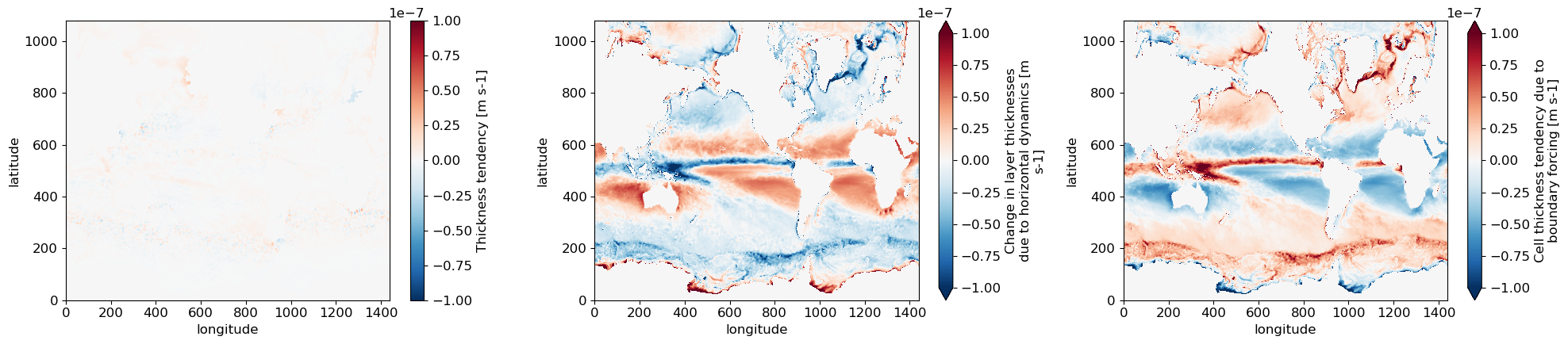
[3]:
fig, axes = plt.subplots(1,3, figsize=(20, 4.5))
ds['dhdt'].plot(ax=axes[0], vmin=-1e-7, vmax=1e-7, cmap="RdBu_r")
ds['dynamics_h_tendency'].plot(ax=axes[1], vmin=-1e-7, vmax=1e-7, cmap="RdBu_r")
ds['boundary_forcing_h_tendency'].plot(ax=axes[2], vmin=-1e-7, vmax=1e-7, cmap="RdBu_r")
for ax in axes:
    ax.set_title("")
    ax.set_xlabel("longitude")
    ax.set_ylabel("latitude")
plt.tight_layout()
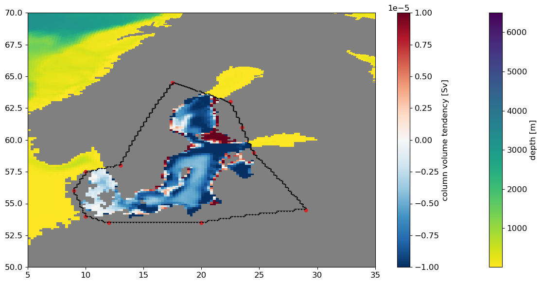
Define a region of interest
We define an arbitrary close sub-region of the domain defined by an irregular polygon, zooming in on the Greater Baltic Sea region analyzed in Drake et al. 2025.
[4]:
name = "Baltic"
lons = np.array([13, 10, 9.0, 10., 12, 20.,  29., 24.5, 23.5, 22.5, 17.5])
lats = np.array([58, 57.5, 56, 54, 53.5, 53.5, 54.5,  59.,  61.,  63., 64.5])
region = reg.GriddedRegion(name, lons, lats, grid)
[5]:
dhdt_dynamics = ds['dynamics_h_tendency']*ds['areacello']*1.e-6

plt.figure(figsize=(12, 6))
plt.subplot(facecolor="grey")
pc = plt.pcolormesh(
    ds['geolon'], ds['geolat'],
    dhdt_dynamics.where(region.mask).where(dhdt_dynamics!=0.).squeeze(),
    alpha=1.0, cmap="RdBu_r", vmin=-1e-5, vmax=1e-5
)
pc_dep = plt.pcolormesh(ds['geolon'], ds['geolat'], ds.deptho.where(~region.mask).where(ds.deptho!=0), cmap="viridis_r")
plt.plot(lons, lats, "C3o", markersize=5)
plt.plot(reg.loop(region.lons_c), reg.loop(region.lats_c), "k-", linewidth=0.5)
plt.plot(region.lons_uv, region.lats_uv, "k.", markersize=2.)
plt.colorbar(pc_dep, label="depth [m]")
plt.colorbar(pc, label="column volume tendency [Sv]")
plt.xlim(5, 35)
plt.ylim(50, 70)
plt.tight_layout()
Verifying the 2D (vertically-integrated) Divergence Theorem
The specific thickness equation in Boussinesq configurations of MOM6 is given by \begin{equation} \partial_{t} h + \nabla_{r} \cdot (\mathbf{u} h) + \delta_{r}(z_{r} \dot{r}) = \dot{h}. \end{equation}
Integrating in \(z\) and over a region \((x,y)\in \mathcal{R}\) (like the sub-domain defined above), the volume budget is \begin{equation} \partial_{t} \mathcal{V} = \iint_{\mathcal{R}} - \nabla \cdot \mathbf{U} \, \text{d}A + \dot{\mathcal{V}}. \quad\quad\text{where }\mathbf{U} \equiv \int \mathbf{u} h \,\text{d}z \end{equation}
Applying the divergence theorem, we can rewrite the thickness advection term as \begin{equation}
\iint_{\mathcal{R}} -\nabla \cdot \mathbf{U} \, \text{d}A = \int_{\partial \mathcal{R}} \mathbf{U} \cdot \mathbf{n}_{in} \,\text{d}l \equiv \Psi,
\end{equation} with \(\Psi\) the horizontally convergent volume transport, integrating along the region’s boundary \(\partial \mathcal{R}\). Evaluating the LHS area integral is straightforward–just apply a Boolean mask to the diagnosed dynamical thickness tendency term. For the RHS boundary integral term, however, we have to accumulate the normal velocities (e.g. with positive consistently defined inwards) along the region’s boundary. This is more more complicated process, but is
achieved thanks to regionate’s companion package `sectionate <https://github.com/hdrake/sectionate>`__.
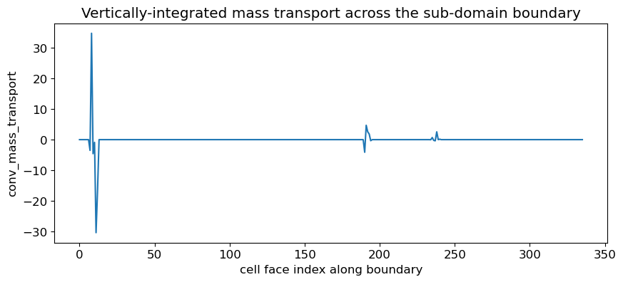
We now compute both sides of the equation and check whether they are self-consistent (within machine precision).
[6]:
Ψ0_tend = dhdt_dynamics.where(region.mask).sum(['xh', 'yh']).values # LHS

Tconv = sec.convergent_transport(grid, region.i_c, region.j_c, layer="z_l", interface="z_i")
Ψ = Tconv['conv_mass_transport'].cumsum("sect").sel(z_l=ds.z_l[::-1]).cumsum('z_l').sel(z_l=ds.z_l[::-1]).compute() # kg/s
Ψ0 = Ψ.isel(sect=-1, z_l=-1).values/rho0*1.e-6 # RHS

print(f"Check whether the discrete Divergence Theorem holds: {np.isclose(Ψ0, Ψ0_tend, rtol=1.e-6, atol=0)}") # single precision floating point
Check whether the discrete Divergence Theorem holds: [[ True]]
We can close the budget to single-precision floating point (float32) precision, which is the best we can hope for given the precision of our diagnostics.
[7]:
plt.figure(figsize=(10, 4))
(Tconv['conv_mass_transport']/rho0*1e-3).plot()
plt.title("Vertically-integrated mass transport across the sub-domain boundary")
plt.xlabel("cell face index along boundary");
[ ]:
[ ]: