Corner case: bipolar grid fold

Examples of challenging test case are regions that cross periodic boundaries or OM4’s Arctic bipolar fold.

# Import packages
import numpy as np
import xgcm
import xarray as xr
import sectionate
import regionate
import matplotlib.pyplot as plt

0. Load data

from load_example_model_grid import load_MOM6_zint_heat_budget
grid = load_MOM6_zint_heat_budget()
ds = grid._ds

File 'MOM6_global_example_vertically_integrated_heat_budget_v0_0_6.nc' already exists at ../data/MOM6_global_example_vertically_integrated_heat_budget_v0_0_6.nc. Skipping download.

We want to must verify that the diagnosed advective heat tendencies (flux convergence) are column-wise consistent with the convergence computed offline from fluxes on the cell faces.

dheatdt_dynamics = (ds['T_advection_xy']*ds['areacello']).sum('z_l')
dheatdt_dynamics = dheatdt_dynamics.where(dheatdt_dynamics!=0.)

plt.figure(figsize=(16, 4.5))
plt.subplot(1,3,1)
dheatdt_dynamics.plot(robust=True)
plt.title("T_advection_xy [volume integral]")

T_adv_heating = -(grid.diff(ds['T_adx'].sum("z_l"), "X") + grid.diff(ds['T_ady'].sum("z_l"), "Y"))
plt.subplot(1,3,2)
T_adv_heating.plot(robust=True)
plt.title("Convergence of (T_adx, T_ady) [surface integral]")

plt.subplot(1,3,3)
(dheatdt_dynamics-T_adv_heating).plot(robust=True)
plt.title("Difference");
plt.tight_layout()

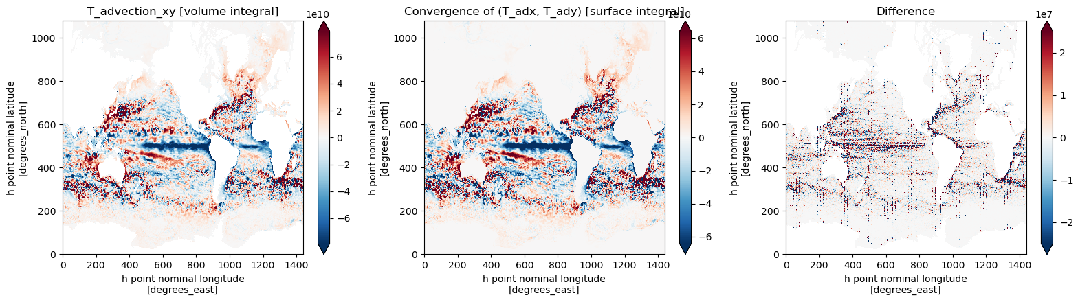
These relative errors are on the order of 10\(^{-5}\), which is consistent with the single precision format of the outputs.

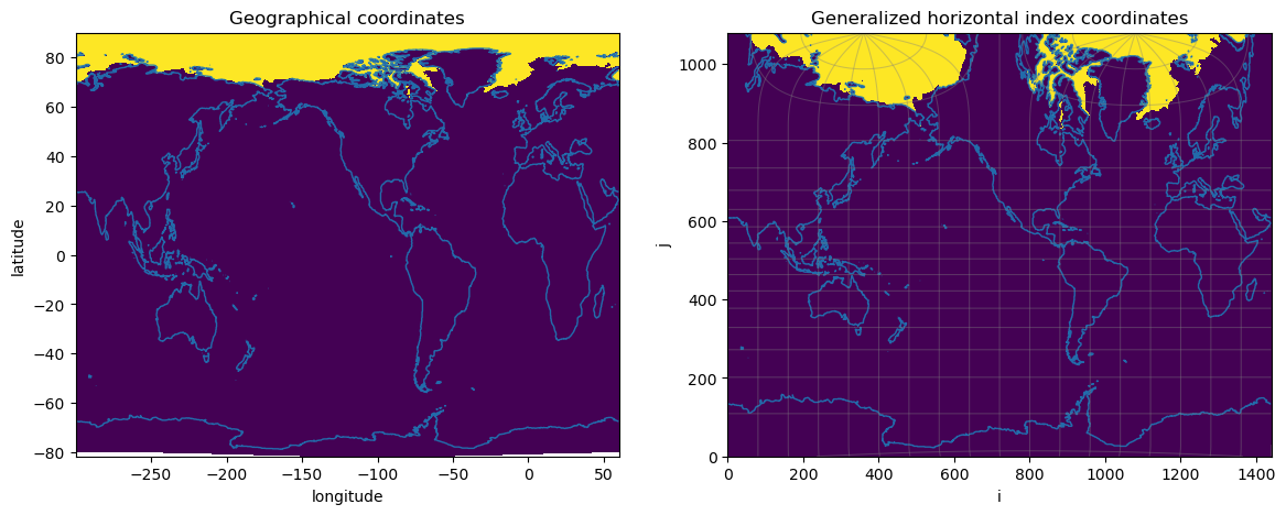
1. Determine a mask for the region of interest.

Let us consider the heat budget for the coldest regions of the high arctic (excluding the Southern Ocean), which have an annual-mean temperature that is below the freezing point of 0ºC (for freshwater at surface air pressure).

ds['mask'] = (
    (ds['tos'].squeeze() < 0.) &
    (ds['geolat'] > 0)
)
plt.figure(figsize=(14, 5))
plt.subplot(1,2,1)
plt.pcolor(
    ds.geolon_c,
    ds.geolat_c,
    ds.mask,
    vmin=0.2, vmax=1.
)
plt.contour(
    ds.geolon,
    ds.geolat,
    ds.deptho,
    levels=[0.],
    colors="C0",
    linewidths=1.,
    alpha=0.9
)
plt.title("Geographical coordinates")
plt.xlabel("longitude")
plt.ylabel("latitude")

plt.subplot(1,2,2)
plt.pcolor(
    ds.mask
)
plt.contour(
    ds.deptho,
    levels=[0.],
    colors="C0",
    linewidths=1.,
    alpha=0.9
)
dlon=20.
plt.contour(
    ds['geolon_c'],
    colors="grey",
    linestyles="solid",
    linewidths=0.75,
    alpha=0.4,
    levels=np.arange(-300., 60.+dlon, dlon)
)

dlat = 10.
plt.contour(
    ds['geolat_c'],
    colors="grey",
    linestyles="solid",
    linewidths=0.75,
    alpha=0.4,
    levels=np.arange(-90., 90.+dlat, dlat)
);
plt.title("Generalized horizontal index coordinates")
plt.xlabel("i")
plt.ylabel("j");

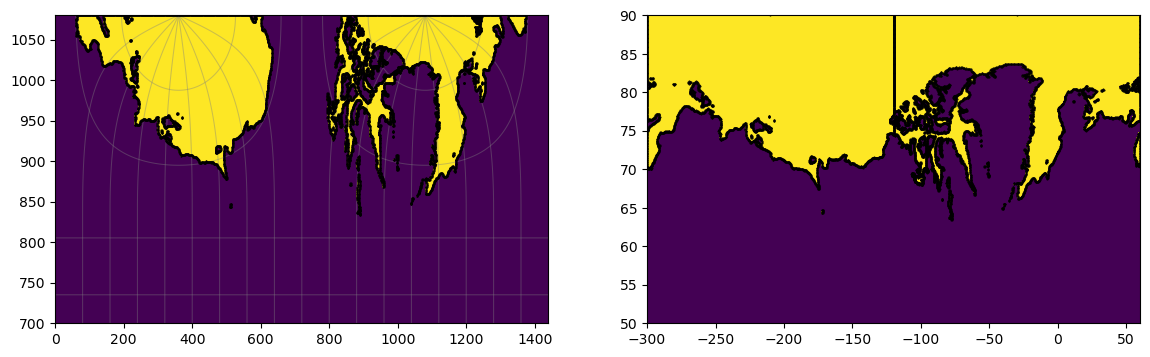
2. We use regionate to find the sections that bound the region

On the backend, this approach uses countourpy to find the demical indices of the contours of the mask in index space, and then convert these into the corresponding integer indices of the ocean model’s vorticity grid (corners of C-grid tracer cells).

from regionate import MaskRegions
region_dict = MaskRegions(ds.mask, grid).region_dict

We plot both the indices and geographical coordinates to verify that these points indeed exactly bound the mask.

Note: Because of the tripolar grid folds at high latitudes, regionate splits the mask in two (as seen by two separate large regions in index space, which are adjacent but separate by a vertical line of indices in geographical coordinates. This does not affect our estimates of the transport, however, because the two sets of fluxes normal to the fold are exactly opposite, and thereby cancel when added together (as below).

plt.figure(figsize=(14, 4))
plt.subplot(1,2,1)
plt.pcolor(
    region_dict[0].mask,
)
dlon=20.
plt.contour(
    ds['geolon_c'],
    colors="grey",
    linestyles="solid",
    linewidths=0.75,
    alpha=0.4,
    levels=np.arange(-300., 60.+dlon, dlon)
)

dlat = 10.
plt.contour(
    ds['geolat_c'],
    colors="grey",
    linestyles="solid",
    linewidths=0.75,
    alpha=0.4,
    levels=np.arange(-90., 90.+dlat, dlat)
);

plt.ylim(700, None)
for p, region in enumerate(region_dict.values()):
    plt.plot(region.i_c, region.j_c, "k.", markersize=1)

plt.subplot(1,2,2)
plt.pcolor(
    ds.geolon_c,
    ds.geolat_c,
    region_dict[0].mask,
)
plt.ylim(50, None)
for p, region in enumerate(region_dict.values()):
    plt.plot(region.lons_c, region.lats_c, "k.", markersize=1)

print(f"""
While the region is mostly made up of two large closed sub-regions (in index space),
there are actually {len(region_dict)-2} other smaller regions that make up external islands
or internal holes in the mask! This method also carefully takes each of those into account.""")

While the region is mostly made up of two large closed sub-regions (in index space),
there are actually 123 other smaller regions that make up external islands
or internal holes in the mask! This method also carefully takes each of those into account.

3. We use sectionate to compute the advective heat fluxes that converge into the region.

total_convergent_heat_transport = 0.

for p, region in enumerate(region_dict.values()):
    ds_sec = sectionate.convergent_transport(
        grid,
        region.i_c,
        region.j_c,
        utr="T_adx",
        vtr="T_ady",
        layer="z_l",
        interface="z_i",
        outname="conv_heat_transport",
        positive_in=region.mask,
    )

    region.convergent_heat_transport = ds_sec['conv_heat_transport'].sum("z_l").isel(time=0).compute()

    total_convergent_heat_transport += region.convergent_heat_transport.sum(["sect"]).values

print(f"The total advective heat convergence into these cold regions of the Arctic is: {total_convergent_heat_transport*1e-12} TW")

The total advective heat convergence into these cold regions of the Arctic is: 38.724284716604 TW

4. We verify our calculation by comparing against the volume integral of the masked tendency terms

dheatdt_dynamics = (ds['T_advection_xy']*ds['areacello']).sum('z_l')
dheatdt_dynamics = dheatdt_dynamics.where(dheatdt_dynamics!=0.)

advective_heating_rate = dheatdt_dynamics.where(region_dict[0].mask).sum(["xh", "yh"]).isel(time=0).values

percent_error = np.round(np.abs((total_convergent_heat_transport - advective_heating_rate)/advective_heating_rate)*100, 4)
print(f"""
Our calculation of the total heat flux converging into the region is within {percent_error}%
of the {advective_heating_rate*1e-12} TW value computed from the more direct advective heat tendency diagnostic,
giving us confidence in our calculations.
""")

Our calculation of the total heat flux converging into the region is within 0.0011%
of the 38.72470118125829 TW value computed from the more direct advective heat tendency diagnostic,
giving us confidence in our calculations.

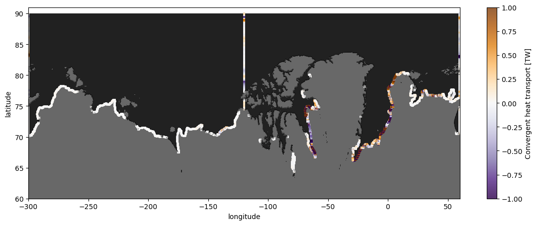
5. The pay-off: understanding advective tendencies by tracing them back to boundary fluxes

Where this flexible convergent-flux-integral approach becomes powerful is when we unravel the cross-boundary integral to reveal the spatial (and temporal) pattern of the heat fluxes into the region. This is a particularly powerful tool for oceanographic problems, where very strong anisotropies due to bathymetric variations, surface forcings, and emergent dynamical structures (boundary currents, jets, eddies, etc.) cause fluxes to vary several orders of magnitude and are often dominated by a few localized hot spots.

Below, we visualize the spatial structure of the heat fluxes into the biggest of the sub-regions.

vmax = 1
plt.figure(figsize=(14,5))

plt.pcolor(
    ds.geolon_c,
    ds.geolat_c,
    region_dict[0].mask,
    cmap="Greys",
    vmin=-3, vmax=1.5
)

for p, region in enumerate(region_dict.values()):
    if len(region.lons_c) < 100: continue
    plt.plot(
        region.convergent_heat_transport['lon'].where(region.convergent_heat_transport==0.),
        region.convergent_heat_transport['lat'].where(region.convergent_heat_transport==0.),
        "k-", lw=1., alpha=0.4
    )
for p, region in enumerate(region_dict.values()):
    if len(region.lons_c) < 100: continue
    sc = plt.scatter(
        region.convergent_heat_transport['lon'],
        region.convergent_heat_transport['lat'],
        c = ((region.convergent_heat_transport*1e-12)
             .where(region.convergent_heat_transport!=0.)),
        marker="s",
        s = 10,
        cmap="PuOr_r",
        vmin=-vmax,
        vmax=vmax,
        edgecolor="k",
        linewidth=0.,
        alpha=0.8
    )

plt.colorbar(sc, label="Convergent heat transport [TW]")
plt.ylabel("latitude")
plt.xlabel("longitude");
plt.ylim(60, 91);